LLM Cost Optimization in Bifrost: Part 1

Introduction

AI costs at enterprises can become expensive quickly. Recent examples show this clearly - Uber reportedly exhausted its annual AI budget only four months into 2026, while Pylon’s CEO said the company’s Anthropic bill was set to jump from $400K to $1.4M a year after crossing 150 seats. These are different companies at different scales, but the pattern is similar: once AI usage becomes normal across teams, cost control becomes an operational problem, not just a pricing problem. Most teams start by looking at the obvious parts of the bill : model pricing, repeated unnecessary prompts, and whether caching is enabled and actually getting cache hits (model changes in the middle of a codex/claude code session breaks the cache) These things indeed matter, but they are only part of the problem.

In practice, token usage is affected by many smaller decisions. Questions like which model handles a request? How much tool context gets sent with every agent call? Is reasoning enabled for requests that do not need it? Are there budgets and limits in place before usage grows, etc. Bifrost handles these decisions at the gateway layer. Since every request already passes through the gateway, it becomes a natural place to apply caching, routing, reasoning controls and governance consistently. This post is the first part of a series on token cost optimization in Bifrost. We will start with the main areas where token cost builds up, and how gateway level controls can reduce unnecessary spend.

The first layer is the simplest one: avoid paying twice for work the model has already done. That is where semantic caching comes in.

Semantic caching

A good first place to reduce token cost is identical or semantically similar requests that can be served without another LLM provider call. The user prompt’s wording may change, but the request can still be close enough to reuse a previous response.

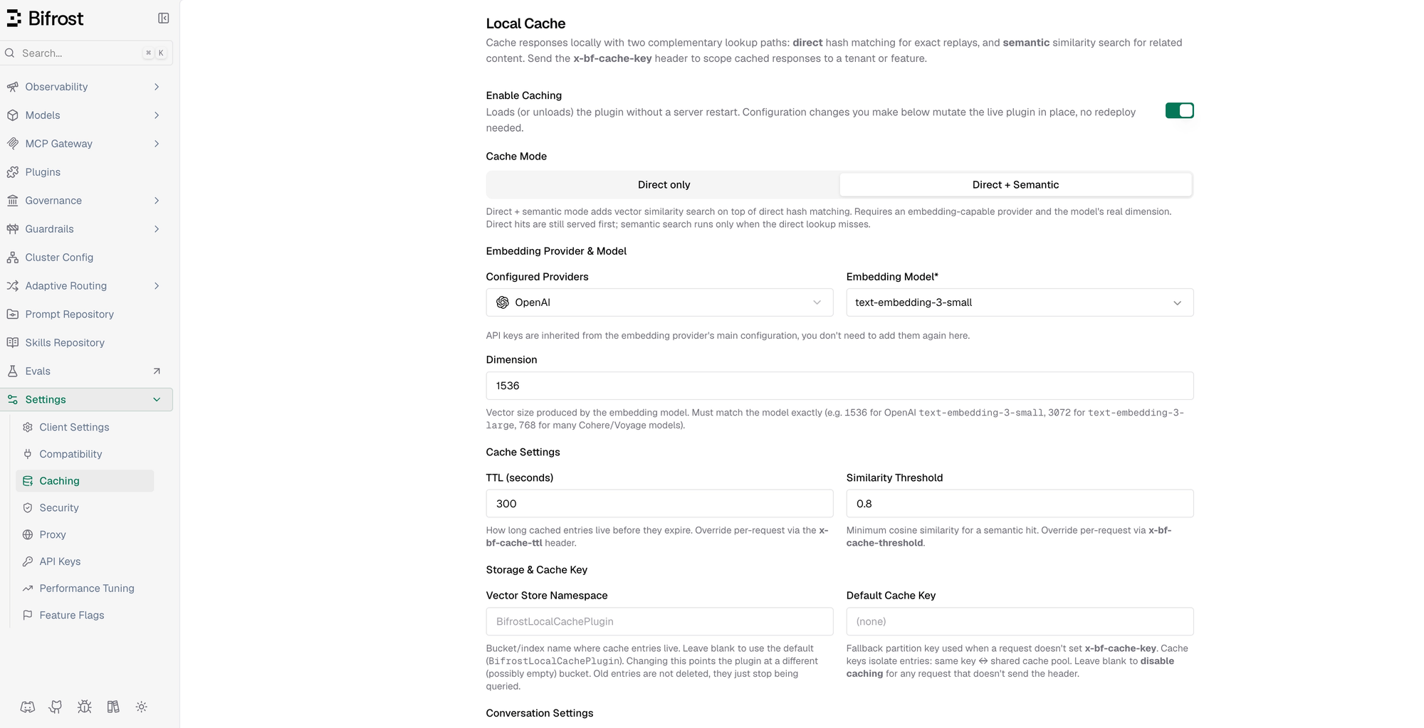
Bifrost's semantic caching supports two cache modes. The first layer is Direct mode, which uses a hash match to catch exact repeats without generating embeddings. This keeps the lookup cheap for requests that are byte-for-byte the same. The second is Direct + Semantic mode, this mode keeps the same direct hash match first, but if there is no exact match, uses semantic similarity over embeddings. This catches near repeats that a hash match would miss, such as “how do I reset my password?” and “I forgot my password, what do I do now?”. It can also reduce latency if we do find a similar match.

The defaults are designed to work without much setup : a similarity threshold of 0.8, a five minute TTL (how long cached entries live before they expire) and 1536 - dimension embeddings from text-embedding-3-small. These settings can also be overriden per request through headers, because caching policy is not the same for every workflow. A support FAQ can usually use a looser cache policy while a high stakes workflow may need a tighter threshold and shorted TTL.

Semantic caching is indeed useful, but it has a natural ceiling. It only helps when the same or similar requests appears again. As for provider side prompt caching, small changes in context/prefix makes it miss the cache (even adding a new mcp tool in the middle of the conversation), the result is that you will be charged for processing the entire prompt of tokens again. That is why caching is the first layer of token cost optimization, not the whole strategy.

MCP Code Mode

Semantic caching helps when similar requests repeat, but agents have another large source of token usage : the tool definitions of the tools attached. Modern agents often connect to multiple MCP servers. Each server exposes tools, and those tool definitions are usually serialized into the model’s context on every LLM call. If an agent is connected to several MCP servers, it can end up sending hundreds of tool schemas with each request, even when the task only needs one or two of them. That creates additional cost before the model has generated any output. The model receives more context each turn, the provider processes more input tokens, and the application pays for tool definitions that may not be used.

MCP Code Mode changes this access pattern. Instead of sending every tool definition into context upfront, Bifrost exposes four meta-tools that let the agent discover and load tools as needed. The agent can list available tool files, read only the relevant ones, pull documentation on demand, and execute orchestration logic in a sandboxed Starlark program. The result is that tool access becomes more selective. The model still has a way to use the tools it needs, but it does not need to carry the full tool surface area in context on every request.

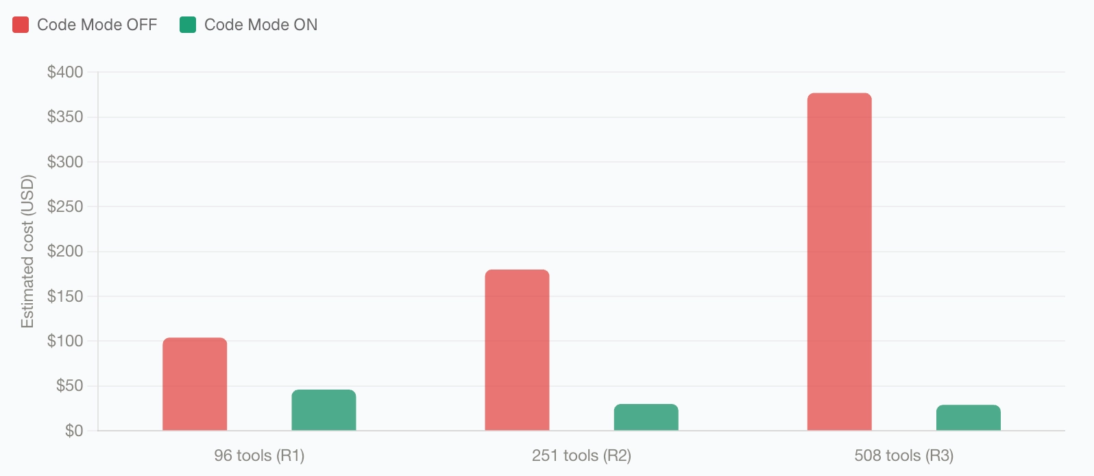
In our internal benchmark with 508 tools across 16 MCP servers, token usage dropped from 75.1 million tokens to 5.4 million tokens, a 92.8% reduction. Estimated cost went from $377 to $29. The pass rate stayed at 100%, which is the important part: the benchmark did not reduce cost by removing the agent’s ability to complete tasks. It reduced cost by changing how tool context was loaded.

Complexity-based routing

Many AI Applications start with one default model for most requests. It is simple to configure, but it also means the same model handles everything: simple clarifications, brainstorming requests, summarization, coding tasks, and deeper reasoning requests. The application works, but many requests end up paying for more model capability than they actually need.

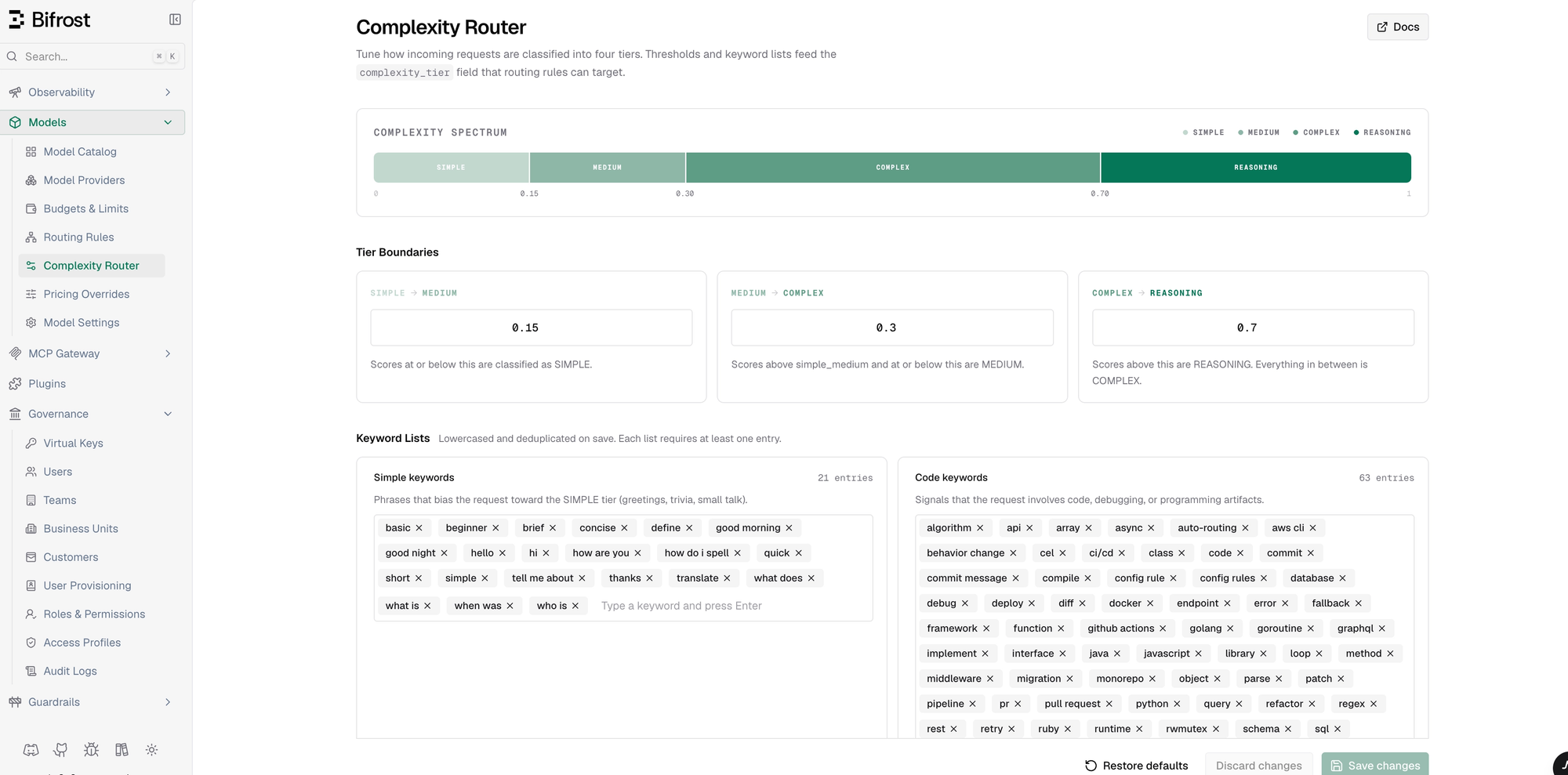
Bifrost’s complexity router helps split that traffic by request difficulty. It scores each incoming request and assigns it to one of four tiers: simple, medium, complex, or reasoning. The scoring is fast and deterministic - exact keyword matching along with signals like code content, reasoning markers, technical terms, and token count. It does not require an extra model call to decide where the request should go.

That tier is exposed as complexity_tier, which can be used in routing rules in Bifrost. For example, simple requests can go to a smaller, faster model like gpt-5.4-nano, medium requests can use a mid-tier model, complex requests can use a stronger model, and reasoning-heavy requests can be reserved for a reasoning model. The goal is not to lower quality. The goal is to stop sending every request to the most expensive path by default.

The scoring is configurable. Tier boundaries and keyword lists can be tuned for your usecase, because complexity signals are not the same everywhere. A term that matters in a legal review workflow may be normal background noise in a coding agent. The defaults are meant to work as a starting point, but teams should adjust them based on the traffic they actually see.

Complexity routing also works alongside Bifrost’s adaptive load balancing. The routing rule decides what kind of model should handle the request. Load balancing then chooses the healthiest available route for that model class based on signals like errors, latency, and utilization. In other words, complexity routing handles cost and capability fit; load balancing handles route health.

Reasoning budget control

Reasoning models can spend a large number of tokens before producing the final answer. That is useful for genuinely hard tasks, but wasteful for requests like basic summarization.

The challenge is that reasoning controls are not consistent across providers. OpenAI exposes reasoning through effort levels, while Anthropic and other providers may expose token budgets or different provider-specific parameters. Without a gateway-level abstraction, each application has to know how to configure reasoning for each provider separately.

Bifrost normalizes this control at the gateway. Callers can set reasoning parameters on the request, and Bifrost maps them to the right provider-specific format. Effort levels map to budget ratios, from roughly 2.5% of the budget for minimal effort up to 80% for high effort. Reasoning can also be turned off entirely for requests that do not need it.

The useful part is consistency. Instead of every caller remembering the right reasoning parameter for each provider, the gateway gives callers one common request shape across providers. Teams can keep reasoning available where it helps, while avoiding it as a default cost on requests that do not need it.

Governance, budgets, and visibility

Cost optimization does not stop after caching, routing, and reasoning controls are configured. The usage changes over time. New teams get onboarded, new virtual keys are created, agents start using more tools, and traffic shifts across providers. Without budgets and limits, cost can creep back even if the initial setup was efficient.

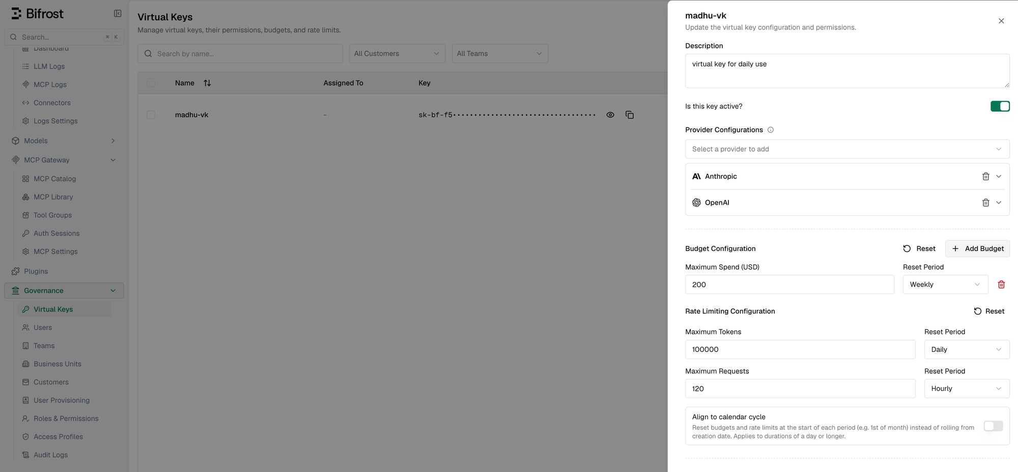
Bifrost’s governance layer gives teams a way to enforce those limits at multiple levels. Budgets can be set independently for customers, teams, virtual keys, and provider configs. When a request comes in, Bifrost checks the applicable budgets in the hierarchy, and each one has to pass before the request is allowed. That means a virtual key or provider config can hit its own limit before it affects the larger team or customer budget.

Rate limits work alongside budgets. Bifrost supports both request limits and token limits, so teams can control not just how many calls are made, but also how much token volume flows through a key or provider over a period of time. Provider-level limits are useful when different providers have different cost profiles, capacity limits, or fallback roles.

The cost calculation also accounts for the things that change the final bill, including provider pricing, token usage, request type, cache status, and batch operations. That matters because the limits should be based on the cost the system is actually incurring, not just raw request counts.

This is also where visibility matters. Per-key and per-provider usage views make it easier to see which teams, workflows, or providers are driving spend. Without that, teams are left guessing where the next cost issue is coming from. With it, cost control becomes part of the operating model instead of a one-time optimization pass.

Conclusion

So LLM cost is not one problem with one fix. The way we think about token cost optimization in Bifrost is simple: reduce unnecessary work before the request reaches the provider.

Taken together, these controls cover different parts of the same request path: whether the provider needs to be called, how much context is sent, which model handles the request, how much reasoning is allowed, and what limits apply once usage grows.

The gateway is where these decisions fit naturally, because every request already passes through it. Instead of handling cost controls separately in every application, Bifrost can apply them in one place.

The MCP Code Mode benchmark is a good example of this. The 92.8% token reduction did not come from paying less for the same tokens. It came from sending fewer unnecessary tokens in the first place.